
|
|
COMPUTATIONAL FLUID DYNAMICS
INTRODUCTION Introduction to Computational Fluid Dynamics
FREE SURFACE FLOWS
VOF-BASED ALGORITHMS
INTRODUCTION
CFD provides numerical approximation to the equations that govern fluid motion.
Application of the CFD to analyze a fluid problem requires the following steps.
First, the mathematical equations describing the fluid flow are written. These are
usually a set of partial differential equations. These equations are then discretized
to produce a numerical analogue of the equations. The domain is then divided into small
grids or elements. Finally, the initial conditions and the boundary conditions of the
specific problem are used to solve these equations. The solution method can be direct
or iterative. In addition, certain control parameters are used to control the convergence,
stability, and accuracy of the method.
Back to the top
FREE SURFACE FLOWS
PowerPoint Presentation on Free Surfaces
Free surface flows refer to flows where there is an
interface between a gas and a liquid with a large density difference.Due to a low density, the inertia of the gas is
usually negligible, and the only influence of the gas is its pressure acting on the interface. The liquid can thus move
freely, and the locations of the free surface must be determined as part of the solution process.
One method to model a free surface is to construct a Lagrangian grid that moves with the fluid. The Lagrangian method has
the advantage of
tracking the free surface automatically, but fails
to model flows with large amplitude surface motions due to
serious deterioration of the mesh. The Arbitrary Lagrangian
Eulerian (ALE) method is thus introduced with a proper
regridding techniques. Still, these methods can not
successfully handle complex free surface flows involving
surface folding and merging. One of the early methods that can
handle surface folding and merging is the
Marker-and-Cell (MAC) method. The MAC method involves
a Lagrangian particle movement and an Eulerian flow
field calculation. The marker is used to track the centroid
of the fluid element. Its velocity is obtained by
averaging the Eulerian velocities in its
vicinity. This method, however, suffers from an
artificial creation of high or low marker
number densities due to the irregularity of the flow
field, such as in the converging and diverging flows and stagnation flows.
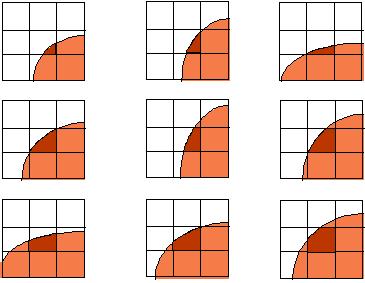
Based on a concept of a fractional volume of fluid, the volume of fluid (VOF) method is developed to follow the
free surface with the volume-tracking feature of the MAC method but without its large memory and CPU costs.
In this approach, only one
storage word is required for each element (or cell), namely,
the volume fraction, f. Consider an Eulerian structured grid and
an actual curved interface cutting through it. Assume that this
curve is the free surface of a liquid domain in a 2-D flow field.
Therefore, one can define a volume fraction field in this mesh,
f, that can take values between 1 and 0. That is, f=0 represents
a cell without liquid (empty cell), f=1 a "full cell," and
0
Back to the top
VOF BASED ALGORITHMS
We have developed a series of method for the interface advection. These are as follows:
- FLAIR
PowerPoint Presentation on FLAIR Algorithms
- FEM-VOF
PowerPoint Presentation on FEM-VOF
- HFM
- SFM
- CLEAR-VOF
There are three basic approaches involved in
FEM and Free Surface Flow. These are:
1) Fixed mesh and free boundary is tracked
2) Deformed spatial mesh using a 3-stage iterative cycle
- Stage 1: Assume shape of free boundary
- Stage 2: BVP solved after discarding 1 BC on free boundary
- Stage 3: SHape of boundary is updated using previously neglected BC
- Cycle is repeated until convergence is achieved
3) Deformed mesh and define nodes on free boundary
- Nodes give extra degrees of freedom
- Field variables and boundary position solved simultaneously using a Newton-Rapson iterative procedure
We combine the FEM and VOF techniques because
- FEM solves for the field variables on a deforming boundary
- VOF used to advect the boundary interface
The advantages of this process are:
- Simulation of Large Surface Deformations (i.e. merging and breaking)
- Accurate implementation of boundary conditions
- Increase in computational efficiency
Back to the top
|
|
|
|